Chilling hours: the three models and when each one tells the truth

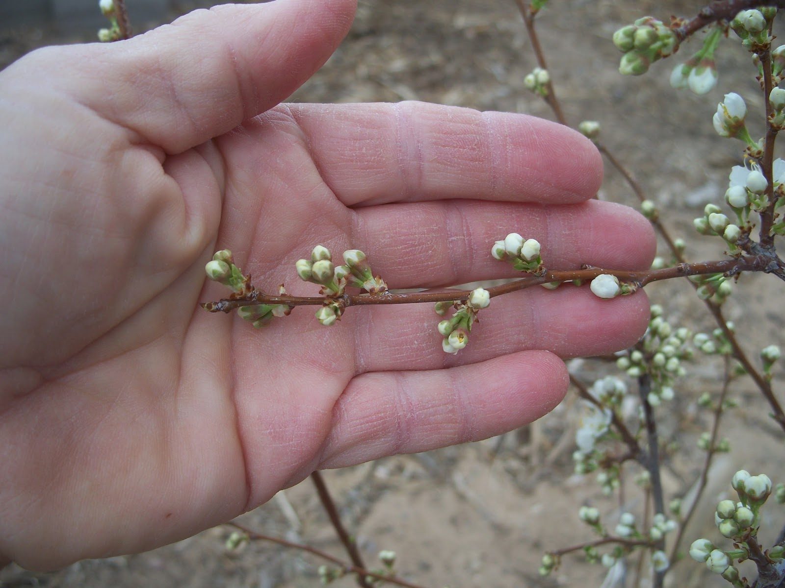
A shoot carrying buds at several different stages of development — Fig. 1On the same shoot there are buds at green tip, buds at white bud and flowers already open. This unevenness is not a trait of the cultivar. It is the visible signature of a winter that did not cover the chilling requirement. The number that describes that winter depends on the model it was measured with.

Savvas Pastopoulos, Agronomist MSc, Pastopoulos Agronomics, Neos Mylotopos, Pella, Greece

“Chilling hours” is not one quantity. It is at least three, with different units, different logic and different reliability depending on the climate and the season. This article explains what each of them measures, which one suits which conditions, and points to the tool that runs all three models on the same data, with no installation and without the data leaving the machine.

Note on units and on scope Temperatures are in degrees Celsius throughout. Chilling Hours, Utah Chill Units and Dynamic Chill Portions are different quantities, not different units of the same quantity, and they cannot be converted into one another by a fixed factor.

3models, three different units

0 to 7.2 °Cthe classic chilling hours window

−1the Utah penalty for every hour above 18 °C

70%the threshold for any dormancy-breaking treatment

Contents

Why a model is needed and a thermometer is not enough
The three models, with their weighting tables
Which model for which climate and which season
What the Greek data show
Where the calculation is done
How the divergence between the three models is read
Where the data come from and when counting starts
Documented requirements by species
Sources

1. Why a model is needed and a thermometer is not enough

Winter dormancy in deciduous fruit trees is endodormancy: the inhibition is internal to the bud and is lifted only by chilling [1]. The question “how much chilling did the orchard get this winter” looks simple but conceals a difficulty: not all low temperatures contribute equally, and high temperatures may negate what has already accumulated. A model is precisely that: a function that converts hourly temperatures into accumulated chill.

Chilling requirements determine where a cultivar can be grown, and failure to meet them leads to reduced and degraded production, and in some cases to abandonment of the crop [2]. With climate change the question has become current again, because districts that were taken for granted no longer are.

Three terms that are constantly confused A Chilling Hour (CH) is one hour within a temperature window. A Chill Unit (CU) is one hour weighted by a factor that may be negative. A Chill Portion (CP) is a unit of an entirely different nature, arising from two-step chemical kinetics, and does not correspond to hours. The three numbers do not convert into one another by a fixed coefficient, because their relationship depends on the temperature distribution of the particular season.

Sources: 1 2

2. The three models, with their weighting tables

2.1 Chilling Hours, the 0 to 7.2 °C model

The oldest and simplest. Every hour with a temperature between 0 and 7.2 °C counts as one chilling hour; anything else counts zero [3] [4]. The 7.2 °C figure is the 45 degrees Fahrenheit of the original study in Georgia, where thresholds of 700, 900 and 1,100 hours were tested [4].

Its basic problem: it subtracts nothing for warmth. A winter with 400 cold hours and ten days at 20 °C in between counts the same as a winter with 400 cold hours and no warm days, although physiologically the two are entirely different.

2.2 Utah Chill Units

The next step, from Utah State University. Each hour is weighted according to its temperature, and high temperatures subtract units [5]:

Temperature of the hour	Units	What it means
up to 1.4 °C	0	Too cold, no contribution
1.4 to 2.4 °C	0.5	Partial contribution
2.4 to 9.1 °C	1.0	The optimum window
9.1 to 12.4 °C	0.5	Partial contribution
12.4 to 15.9 °C	0	Neutral zone
15.9 to 18 °C	−0.5	Negates chill
above 18 °C	−1.0	Negates a full unit

The idea that very low temperatures do not contribute is correct and important: below 1.4 °C the mechanism stops. The problem appears at the other end: the penalty is linear and unforgiving, so in a mild climate the total can fall to zero or even go negative, which is not physiologically tenable.

2.3 Dynamic Chill Portions

The most recent and the most different. It does not sum weights; it describes a two-step chemical process [6] [7]:

Step 1. In the cold an unstable precursor is formed. This is reversible: if it warms up, the precursor is destroyed.
Step 2. Once the precursor reaches a critical amount, it converts irreversibly into one stable chill portion. From then on nothing undoes it.

Why the first step is fragile. The precursor forms in the cold, but while it remains unstable it is not yet banked: a high enough temperature dissolves it and the accumulation goes back. This is exactly where the three models part company. In Chilling Hours nothing is ever subtracted. In Utah it is subtracted linearly and permanently, including chill banked months earlier. In the Dynamic model only what has not yet been fixed is lost, and what has already become a portion is undone by no amount of heat.

The counter-intuitive prediction of the model Because the second-step conversion is favoured by moderately warm temperatures, the model predicts something neither of the other two can: a mild warm spell immediately after cold can increase accumulated chill, by locking the precursor into a permanent form. Only genuinely high temperatures, arriving before the conversion has taken place, destroy the accumulation. This is why alternating cold and mild warmth, that is, the typical Mediterranean winter, performs better than the Utah model calculates.

The unit does not convert into hours. A chill portion is dimensionless: it counts how many times the two-step cycle was completed, not how long it was cold. No coefficient converts it into hours, not even approximately, because the same hour at 6 °C counts differently depending on what came before and after. That is why every cultivar requirement is written together with its model, and why a value in portions is never compared with a value in hours.

The order of magnitude, which is also the easiest error check Hours are counted in hundreds, Utah units in thousands, portions in tens. In the European EUFRIN network a whole winter gave from 45 portions at Murcia in Spain to 97 to 98 at Cuneo and Bucharest [9], and the requirements of two cherry cultivars are 58 and 84 portions [8]. A three-digit figure in portions does not come out of a normal winter. When one appears, the error is in the data or in the unit, not in the winter.

What this means for a Greek winter. Cold nights that build the precursor and mild days that lock it in are precisely the pattern of a Mediterranean winter. Utah counts that pattern as a loss and the Dynamic model counts it as a gain. That is where most of the distance between the two models in a Greek season comes from, and not from measurement error.

Sources: 3 4 5 6 7 8 9

3. Which model for which climate and which season

The answer is not a matter of taste; it has been tested on real data.

Conditions	Most suitable	Why
Cold continental winter, without warm spells	All three agree; Chilling Hours are adequate for practical use	With no warm hours there is nothing to subtract, so the simple sum gives the same picture as the complex models.
Mediterranean winter with alternating cold and warmth	Dynamic	It is the only one that handles the alternation correctly. On ten sweet cherry cultivars in Apulia it outperformed the other three [8].
Mild or warm winter, marginal coverage	Dynamic, by a wide margin	Utah overestimates the destruction of chill and can produce absurdly low or negative totals. Chilling Hours, conversely, overestimate the accumulation.
Comparing years with each other	Dynamic	It gives more homogeneous accumulation across years, so its values are more comparable [9].
Predicting bloom date	Dynamic	On 14 peach and nectarine cultivars at 11 sites in five countries, it gave better predictions than Utah, Positive Utah and Chilling Hours [9].
Older cultivar literature	Necessarily Chilling Hours	Most historical requirement figures were published in hours. To be compared with a measurement, the measurement has to be made in the same model.

What the author of the reference software says himself chillR is the standard package for chill analysis. In the documentation of the first two models, its author writes the same warning twice: “After doing extensive model comparisons, and reviewing a lot of relevant literature, I do not recommend using the Utah Model, especially in warm climates! The Dynamic Model (Chill Portions), though far from perfect, seems much more reliable.” The identical note is repeated for the Chilling Hours model [10].

When the “best” model does not help Two caveats that need stating. First, prediction was less successful for low-chill cultivars than for medium- and high-chill ones [9]. Second, a value in Dynamic chill portions is useless if the cultivar's requirement is known only in hours. The choice of model is not made in the abstract, but according to the model in which the requirement of that particular cultivar is available.

Sources: 8 9 10

4. What the Greek data show

The Department of Deciduous Fruit Trees of ELGO-DIMITRA at Naoussa has calculated chill accumulation for locations in Greece and Cyprus using different models, and publishes a spreadsheet that computes all three models from hourly values [2]. It is the same set of three that the tool follows.

Naoussa also took part in the European EUFRIN network, where accumulation ranged from 45 chill portions at Murcia-Torre Pacheco in Spain to 97 to 98 portions at Cuneo in Italy and Bucharest. Bloom was earliest in the moderately cold regions and 7 to 11 days later in the warmer locations of Rome and Naoussa, an indication that rest completion is delayed there [9].

What this means for central Macedonia Naoussa is not a marginal district; but it is on the warm side of the European range, together with Rome. Semi-lowland sites in Pella and Imathia therefore fall exactly in the range where the choice of model matters: Chilling Hours will show comfortable coverage, Utah will show a deficit, and the truth will be closer to the Dynamic model.

Sources: 2 9

5. Where the calculation is done

The three calculations and their comparison are not inside the article. They live in a separate tool, so that it can be updated without rewriting the text and used without having to read the theory first.

The tool

Chilling hours, units and portions, and insect degree-days (in Greek)

It accepts hourly temperatures or daily minimum and maximum, runs all three models on the same data, and gives the percentage of the requirement met when the cultivar requirement is supplied. It also draws directly from the stations of the National Observatory of Athens, so for the areas covered no copying of data is needed at all.

6. How the divergence between the three models is read

The value of running all three models on the same series is not to find the right number. It is that the distance between them describes the season.

How to read the divergence If hours show comfortable coverage while Utah units collapse, the winter had many warm hours: reality lies in between, closer to the portions. If all three give the same picture, the winter was consistently cold and the model does not matter. A large divergence is not a computational error. It is information about the season.

7. Where the data come from and when counting starts

Sources of hourly temperatures

An on-site weather station or data logger. The best solution, because chill differs substantially over a few kilometres and with elevation. Most loggers record at ten-minute intervals; conversion to hourly values is needed, and a ready-made spreadsheet exists for it [2].
Station networks. Useful, subject to the distance and the difference in elevation from the block.
Daily minimum and maximum. When nothing else is available. The tool accepts this format too, generating hourly values with a sine curve.

Estimating from min and max is not measuring Generating hourly values from daily extremes is an estimate. The real daily course is not sinusoidal: night-time cooling follows a logarithmic curve and the time of the minimum depends on day length. The error is small for Chilling Hours, larger for Utah and most significant for the Dynamic model, which is sensitive to the exact sequence of temperatures. For a planting decision or a treatment, real hourly measurements are needed.

When counting starts

There is no calendar date. The start of accumulation is defined operationally as the date from which chilling hours are recorded consistently [2], in central Macedonia, typically within the second half of November. Counting closes when the cultivar's requirement is met or, in practice, at bud swell.

The only use that justifies the whole exercise The calculation is not an end in itself. It has two practical applications: choosing a cultivar for a site before planting, and determining the 70% of the requirement, which is the threshold below which no dormancy-breaking treatment has a predictable outcome [2]. Anything else is record-keeping.

Sources: 2

8. Documented requirements by species

Values are always given with their model, because without it they mean nothing. None of them was measured in Greece: the general range for sweet cherry comes from literature cited in a Chilean study [11], the values for Burlat and Ferrovia from Apulia in Italy [8], and the values for kiwifruit Hayward from Alabama in the United States [12]. The Greek values come from the Department of Deciduous Fruit Trees at Naoussa [2].

Species and cultivar	Requirement	Model	Source
Sweet cherry, general range	520 to 1,320	Chilling Hours	[11]
Sweet cherry ‘Burlat’, early	58	Dynamic portions	[8]
Sweet cherry ‘Ferrovia’, late	84	Dynamic portions	[8]
Kiwifruit ‘Hayward’	750 to 800	Richardson units	[12]
Kiwifruit ‘Hayward’, adequate budbreak	900	Chilling Hours	[12]
Kiwifruit ‘Hayward’, maximum flowering	1,150	Chilling Hours	[12]

Values for peach, nectarine and apricot under Greek conditions have been published by the Naoussa department and are found in the works listed at source [2]; they are not reproduced here cultivar by cultivar, because those figures are updated and the right thing is to take them from the primary source.

Sweet cherries at fruit set — Fig. 2The same thing, three months later. On a single spur there are fruitlets of different sizes and flowers that did not set, the imprint of a bloom that spread out over time. This is where it is decided whether the count of hours, units or portions described the season correctly.

For the detailed discussion of sweet cherry (requirements, dormancy-breaking agents, the 70% rule and what is permitted in Greece) there is a separate article: Breaking dormancy in sweet cherry. For kiwifruit, where the bud mechanism is entirely different: Kiwifruit bud physiology and flower differentiation.

Sources: 2 8 11 12

9. Sources

The numbers in the text refer to the list below.

[1] Lang, G.A., Early, J.D., Martin, G.C. & Darnell, R.L. (1987). Endo-, para- and ecodormancy: physiological terminology and classification for dormancy research. HortScience 22:371-377. Source for the definition of endodormancy and for the fact that it is lifted only by chilling.
[2] Winter dormancy of deciduous fruit and nut trees. Department of Deciduous Fruit Trees, Institute of Plant Breeding and Genetic Resources, ELGO-DIMITRA, Naoussa, Greece. Source for the consequences of unmet chilling requirements, for the spreadsheet that computes the three models from hourly values, for the definition of the start of accumulation as the date from which chilling hours are consistently recorded, for the 70% threshold, and for the published requirements of Greek cultivars.
[3] Bennett, J.P. (1949). Temperature and bud rest period. California Agriculture 3(11), pp. 9 and 12. Source for the definition of the chilling hour as an hour with a temperature between 0 and 7.2 °C.
[4] Weinberger, J.H. (1950). Chilling requirements of peach varieties. Proceedings of the American Society for Horticultural Science 56:122-128. Source for the 45 °F threshold and for the experimental levels of 700, 900 and 1,100 hours.
[5] Richardson, E.A., Seeley, S.D. & Walker, D.R. (1974). A model for estimating the completion of rest for ‘Redhaven’ and ‘Elberta’ peach trees. HortScience 9(4):331-332. Source for the entire Utah weighting table, with the boundaries 1.4 / 2.4 / 9.1 / 12.4 / 15.9 / 18 °C and the weights 0 / 0.5 / 1 / 0.5 / 0 / −0.5 / −1.
[6] Fishman, S., Erez, A. & Couvillon, G.A. (1987). The temperature dependence of dormancy breaking in plants: mathematical analysis of a two-step model involving a cooperative transition. Journal of Theoretical Biology 124(4):473-483. Source for the two-step mechanism, the unstable precursor and the irreversible conversion.
[7] Erez, A., Fishman, S., Linsley-Noakes, G.C. & Allan, P. (1990). The dynamic model for rest completion in peach buds. Acta Horticulturae 276:165-174. Source for the formulation of chill portions in the form used today.
[8] Palasciano, M. & Gaeta, L. (2017). Comparison of different models for chilling requirements evaluation of sweet cherry cultivars in a Mediterranean area. Acta Horticulturae 1161:405-410. Source for the comparison of four models on ten sweet cherry cultivars in Apulia, for the superiority of the Dynamic model in a Mediterranean climate, and for the values of 58 and 84 portions.
[9] Drogoudi, P., Cantín, C.M., Brandi, F., Butcaru, A., Terrer, J.C., Cutuli, M., Foschi, S., Galindo, A., García-Brunton, J., Luedeling, E. et al. (2023). Impact of chill and heat exposures under diverse climatic conditions on peach and nectarine flowering phenology. Plants 12(3):584. Source for the 45 to 97 to 98 portions across eleven European sites, for the 7 to 11 day delay in Rome and Naoussa, for the superiority of the Dynamic model in both homogeneity and bloom-date prediction over Utah, Positive Utah and Chilling Hours, and for the lower prediction success in low-chill cultivars.
[10] Luedeling, E. chillR: Statistical Methods for Phenology Analysis in Temperate Fruit Trees, source code of the temperature models, CRAN package. Source for the exact parameters and algorithms of the three models as implemented in the tool, and for the author's explicit recommendation against using the Utah and Chilling Hours models in warm climates.
[11] Ardiles, M. & Ayala, M. (2017). An alternative dormancy-breaking agent to hydrogen cyanamide for sweet cherry (Prunus avium L.) under low chilling accumulation conditions in the Central Valley of Chile. Acta Horticulturae 1161:423-430. Source for the range of 520 to 1,320 chilling hours in sweet cherry.
[12] Sibley, J.L., Dozier, W.A., Pitts, J.A., Caylor, A.W., Himelrick, D.G. & Ebel, R.C. (2005). Kiwifruit cultivars differ in response to winter chilling. Small Fruits Review 4(4):19-29. Source for the 750 to 800 Richardson units and for Caldwell's 900 and 1,150 hours in kiwifruit ‘Hayward’.

Photograph: Pastopoulos Agronomics archive.

Disclaimer The tool implements published models and are intended for educational and advisory use. The result depends entirely on the quality of the data entered; values derived from daily extremes are estimates, not measurements. No planting decision, cultivar choice or treatment should rest on them alone. Plant protection products must be used solely in accordance with the approvals in force and the product label; any Greek approvals referred to on this site are those of the Greek Ministry of Rural Development and Food and are valid in Greece only. Any foliar spray carries a risk of marking the fruit and scorching the foliage: a preliminary test on a limited number of trees, with the same product at the same rate, is required, followed by a wait of 5 to 7 days before any general application; spraying is done in the late afternoon or early morning, never in a heatwave and never on foliage under water stress. Every intervention is at the user's own responsibility, following an on-site assessment by a licensed agronomist. Pastopoulos Agronomics accepts no liability for the use of this information.